This work benefited from the valuable help, sources and great advice of Fredrick Bunt (University of Montana). Big thank you Fred!

import xarray as xr
import rioxarray # for the .rio functions
import matplotlib.pyplot as plt
import numpy as np

from pyproj import Transformer
from scipy.interpolate import griddata

Procedures and good habits when writting and reading large geo-spatio-temporal datasets

We deal with large datasets, often time in netCDF format, these datasets span space and time, with associated coordinate systems. Proper handling of those coordinates is essential to reduce error and facilitate user-friendliness, which remains a key component of our work, our science needs to be useful, in perticular to others. Knowledge of the global temperature in ten years is only useful if you can use it to draw conclusions on other processes, in other fields of sciences. This document focuses on proper encoding of the spatial Coordinate Reference System (CRS) and data formatting, based on pre-existing conventions, specifically the NetCDF Climate and Forecast (CF) Metadata Convention.

TL/DR: when encoding a dataset, this one needs a CRS (Coordinate Reference System) encoded along with coordinates in that CRS. A CRS_WKT (Well Known Text) is an efficient way to encode key information in all files. Make sure your datasets have that CRS/proper grid/WKT encoded in, whether it is a model output or a dataset you created for your own use. If you read someone else’s file with a compromised/missing CRS, here are some methods to help you.

ds = xr.open_dataset('/dmidata/projects/nckf/smb_hirham/ANT11_eval_ERA5/1999/01/01/00/ts_sfx_ANT11_ANT11_eval_ERA5_1hr_199901010000-199902010000.nc')
ds

This is an example dataset from an 11km reanalysis of ERA5. I would like to attract your attention on the Dimensions and Coordinates. There are two dimensions here: x and y. Coordinates are that x and y, time and lat and lon. We notice right away that x and y are 1D arrays, vectors in other words, of size 739 and 635 respectively. This indicates a “regular grid”, that can be simply be defined by these two vectors. In other words, one row of that grid will have a single y value, and one column will have a single x value. This regular grid may look exactly like what we need, but we need to make sure that this grid is connected to reality somehow. Indeed, we need to locate this grid with respect to some standards, imagine a coordinate reference system in high school mathematics, you need the coordinates of the origin and its unit vectors. This is the information carried by the CRS, it is a standard way of encoding some coordinate system’s key information, it will usually be latitudes/longitudes or in meters, both having their advantages and inconvenients. Thousands of CRS exist, you can find them on EPSG.io, some will be globally oriented (ex: the modern definition of latitude and longitude is a CRS), some will be more regionally oriented, peticularily the metered CRS (a CRS that uses a unit of meters), they are really accurate at small scale but start being wrong further away from the CRS’s origin due to the curvature of the Earth. There are very simple ways to check one datatset’s CRS:

print(f"Dataset CRS: {ds.rio.crs}")

Dataset CRS: None

This is problematic, there is no CRS encoded here. A common procedure is to have an Attribute called CRS_WKT, standing for Coordinate Reference System Well Known Text, summarizing all the information about the CRS in one spot. More information can be found in the NetCDF CF Metadata Convention document. Here, there is no such attribute because this x/y grid is actually the grid on which the model was run. The format of this dataset is standard (Section 5.2 of the NetCDF CF Metadata Conventions), it is output this way such that no alteration of the data or grid is done and the user can choose to make their own changes. We only have one last source of information: the lat and lon, let’s look at them.

fig,axs = plt.subplots(ncols=2, figsize=(15,6))
ds.lat.plot(ax=axs[0])
ds.lon.plot(ax=axs[1])
axs[0].set_title("Latitute")
axs[1].set_title("Longitude")

Text(0.5, 1.0, 'Longitude')

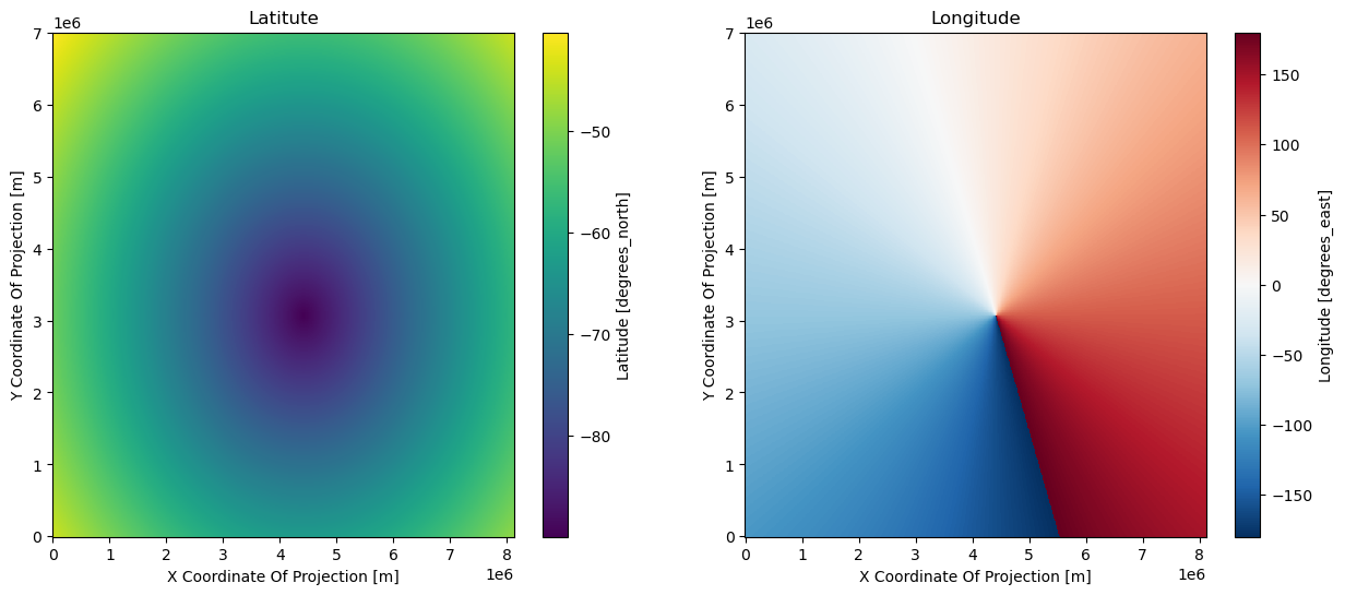
We are in a complex situation where the coordinates that make physical sense, that matter to us, are a 2D grid, which does not function well with xarray and netCDFs. Indeed, we cannot just erase x and y, they are Dimensions and can therefore not be removed, although they have no meaning to anyone else than the person running the model. There are several ways to resolve this.

1: Manually create a grid with appropriate coordinates

We will simply reproject the grid of lat/lon onto a grid that suits us better, but without altering the original dataset. For that exercice, I chose to reproject everything onto a metered CRS centered around Antarctica, the EPSG:3031. This method has the advantage of not compromising the data. Interpolation indeed would affect the data, while reprojecting the grid only affect the location of these data.

transformer = Transformer.from_crs(4326, 3031, always_xy=True)
transformer

<Concatenated Operation Transformer: pipeline>
Description: axis order change (2D) + Antarctic Polar Stereographic
Area of Use:
- name: World
- bounds: (-180.0, -90.0, 180.0, 90.0)

x_reprojected, y_reprojected = transformer.transform(ds.lon, ds.lat)

fig,axs = plt.subplots(ncols=2, figsize=(15, 6))
ds.ts[0].plot(ax=axs[0])
axs[1].pcolormesh(x_reprojected, y_reprojected, ds.ts[0])

## Bonus: finding the x/y of the south pole on the new grid
t = np.unravel_index(np.argmin(ds.lat.values), ds.lat.values.shape)
print(r'Coordinates of the cell closest to the south pole (our grid is 11km spaced, so we are ~4km away from the south pole):', x_reprojected[t], y_reprojected[t])

Coordinates of the cell closest to the south pole (our grid is 11km spaced, so we are ~4km away from the south pole): 4005.7661470373446 -4382.867657798594

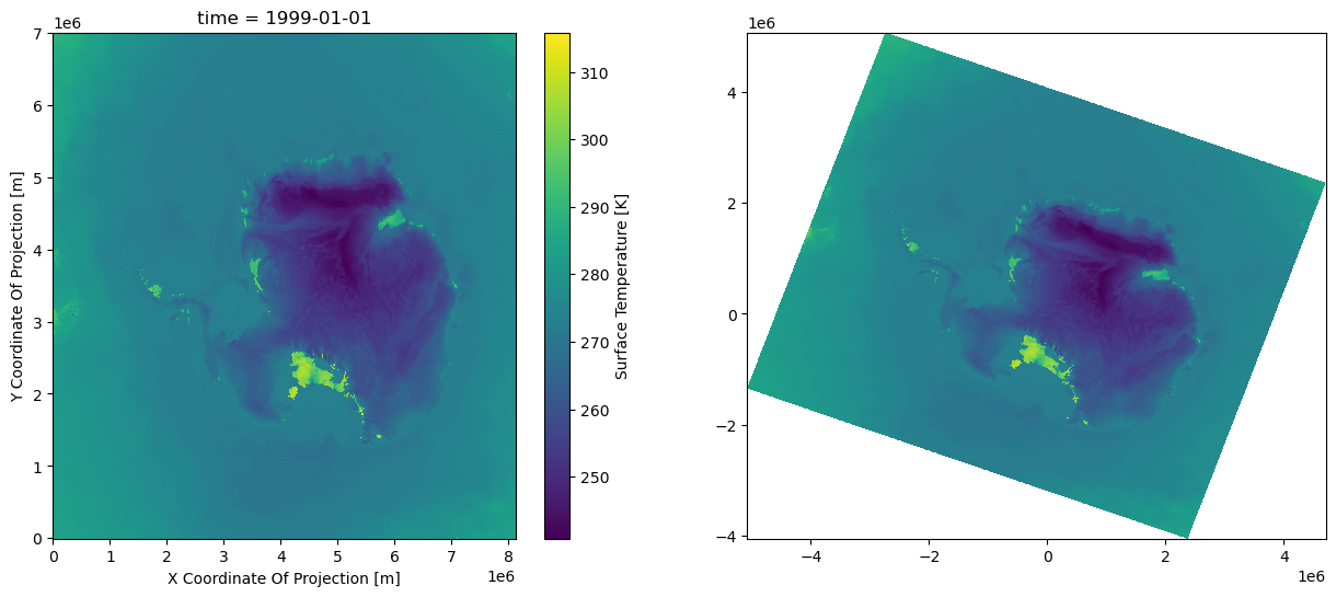
I would like to bring your attention on the following:

• Notice the location of the origin for both grids: 0 is somewhere off in the ocean for the left plot, it is at the south pole in our reprojected grid.
• The orientation: it changed, both Antarctica has been turned but also our grid coordinates are different, shown by the white triangles on the side.
• The scale along one axis: Antarctica has somewhat shrinked on the right plot, although this could be a plotting artifact, this is also the result of distances being appropriately represented after using the lat/lon to meters conversion.

The right plot is closer to a usable grid, we can actual start performing certain tasks using the ´x_reprojected´ and ´y_reprojected´ grids, for example extracting the data at a given location (whether it is lat/lon or meters) very easily.

This method does not affect the data itself, only the location of it, but it takes us away from xarray (example of an extremely powerful and optimised library for this kind of problems), we would like to have a properly set dataset instead of this hybrid numpy/xarray solution, but this only comes at the cost of resampling the data.

######## Bonus: most efficient way to pull data from a list of coordinates:
lat_stations = [-89, -88, -85]
lon_stations = [10,-50,150] # mock numbers

x_stations, y_stations = transformer.transform(lon_stations, lat_stations)

arg_stations = []

for x_, y_ in zip(x_stations, y_stations):
    arg_station = np.argmin(np.ravel(( (x_reprojected-x_)**2 + (y_reprojected-y_)**2)**.5) )   # find the argument of the cell closest to the desired location
    arg_stations.append(np.unravel_index(arg_station, x_reprojected.shape)) 

print('Station indices:', arg_stations)
print('Data at those indices (first time step):', [ds.ts.values[0, *s_] for s_ in arg_stations])

Station indices: [(289, 400), (286, 383), (247, 440)]
Data at those indices (first time step): [254.09996, 256.95547, 255.72516]

2: Resampling the data

If altering the data is not a problem for you; if you want to save the data into your own simple file; if you want to use the full power of xarray on a well organized dataset, you may need to resample the data. To do so, we use the SciPy griddata function.

aspect = ds.y.size / ds.x.size
nx = 700
ny = int(aspect * nx)
shape = (1, ny, nx) # the first dimension is for time
print(f"Target Grid Shape: {shape}")

Target Grid Shape: (1, 603, 700)

A) Building the Target Grid as a Regular Grid

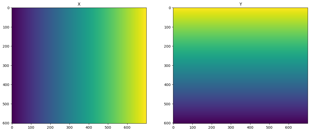
We want a regular grid where every pixel is the same size in x and y. The y coordinates are flipped to follow the common convention of having a decreasing y coordinate for raster data.

x_target = np.linspace(x_reprojected.min(), x_reprojected.max(), nx)
y_target = np.linspace(y_reprojected.min(), y_reprojected.max(), ny)[::-1]
X_target, Y_target = np.meshgrid(x_target, y_target)

fig, axs = plt.subplots(ncols=2, figsize=(15, 6))
axs[0].imshow(X_target)
axs[0].set_title("X")
axs[1].imshow(Y_target)
axs[1].set_title("Y")

Text(0.5, 1.0, 'Y')

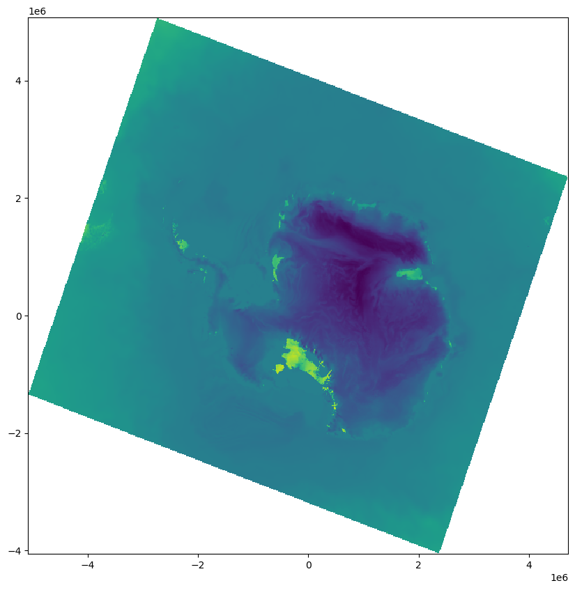
B) Regridding the Data with griddata

We need to interpolate the data onto the target grid.

regridded_data = griddata(
    list(zip(x_reprojected.ravel(), y_reprojected.ravel())),
    ds.ts[0].to_numpy().ravel(),
    list(zip(X_target.ravel(), Y_target.ravel())),
    method="cubic"
)
regridded_data = regridded_data.reshape(shape)

plt.figure(figsize=(10, 10))
plt.pcolormesh(X_target, Y_target, regridded_data[0])

C) Building a New Xarray Object

xdata = xr.DataArray(
    regridded_data,
    dims=("time", "y", "x"),
    coords=(ds.time[:1], y_target, x_target)
).rio.write_crs("EPSG:3031")
xdata

plt.figure(figsize=(10, 8))
xdata.plot(robust=True, cmap="viridis")

print(f"Regridded data CRS: {xdata.rio.crs}")

Regridded data CRS: EPSG:3031

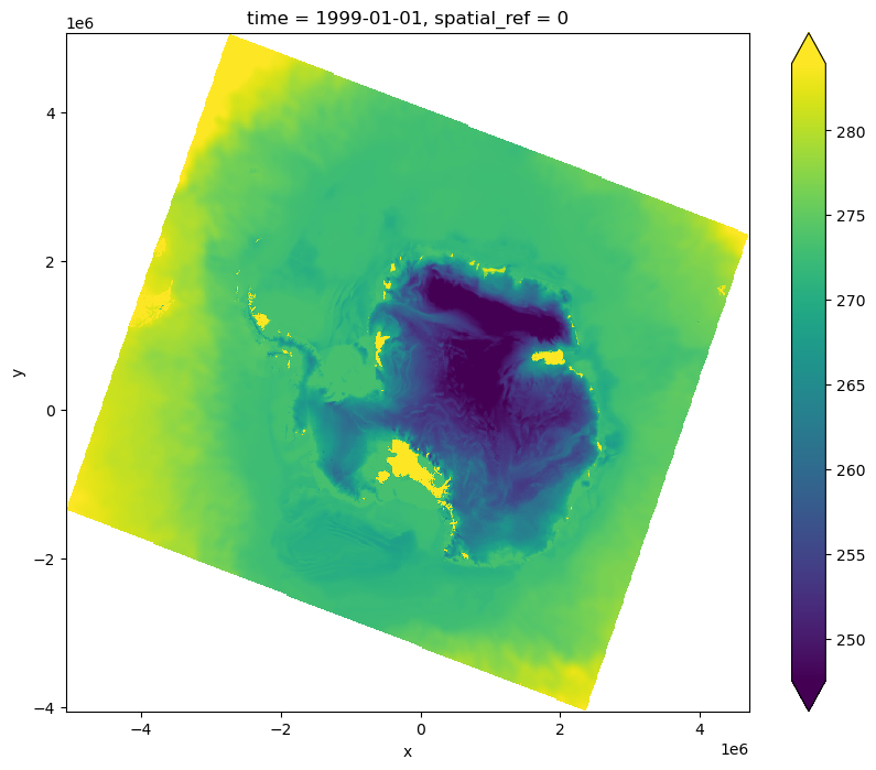
The key point here is that you are able to save this data in a new netCDF file because it has a regular grid. Regular examples from the netCDF or xarray library would suffice to do so.